ABSTRACT
Cloud computing is transforming a large part of the IT industry, as evidenced by the in creasing popularity of public cloud computing services, such as Amazon Web Service, Google Cloud Platform, Microsoft Windows Azure, and Rack space Public Cloud. Many cloud computing applications are bandwidth-intensive, and thus the network bandwidth in formation of clouds is important for their users to manage and troubleshoot the application performance.
The current bandwidth estimation methods originally developed for the traditional Internet, however, face great challenges in clouds due to virtualization that is the main enabling technique of cloud computing. First, virtual machine scheduling, which is an important component of computer virtualization for processor sharing, interferes with packet time stamping and thus corrupts the network bandwidth information carried by the packet timestamps. Second, rate limiting, which is a basic building block of network virtualization for bandwidth sharing, shapes the network packets and thus complicates the bandwidth analysis of the packets.
In this dissertation, we tackle the two virtualization challenges to design new bandwidth estimation methodologies for clouds. First, we design bandwidth estimation methods for networks with rate limiting, which is widely used in cloud networks. Bandwidth estimation for networks with token bucket shapers (i.e., a basic type of rate limiters) has been studied before, and the conclusion is that “both capacity and available bandwidth measurement are challenging because of the dichotomy between the raw link bandwidth and the token bucket rate”.
Our methods are based on in-depth analysis of the multi-modal distributions of measured bandwidths. Second, we expand the design space of bandwidth estimation methods to challenging but not rare networks where accurate and correct packet time information are hard to obtain, such as in cloud networks with heavy virtual machine scheduling. Specifically, we design and develop a fundamentally new class of sequence-based bandwidth comparison methods that relatively compare the bandwidth information of multiple paths instead of accurately estimating the bandwidth information of a single path.
By doing so, our methods use only packet sequence information but not packet time information, and are fundamentally different from the current bandwidth estimation methods that all use packet time information. Furthermore, we design and develop a new class of sequence-based bandwidth estimation methods by conveying the time information in the packet sequence. Sequence-based bandwidth estimation methods estimate the bandwidth information of a path using the time information conveyed in the packet sequence from another path.
CAPACITY AND TOKEN RATE ESTIMATION FOR NETWORKS WITH TOKEN BUCKET SHAPERS
Capacity Estimation
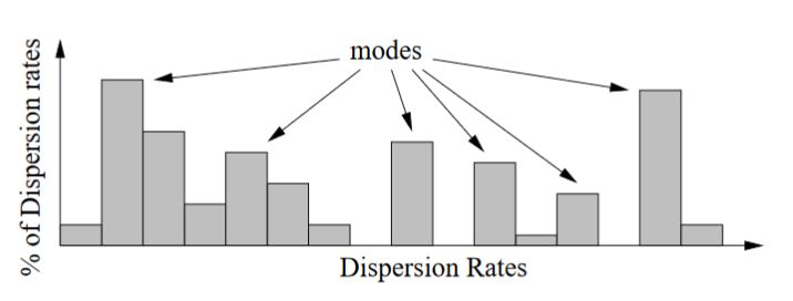
Figure 2.6: Dispersion rate histogram U is multi moda
Figure 2.6 illustrates a possible U. Due to the factors explained in Section 2.4.2, U has multiple modes. A mode is a local maximum (i.e., peak). The strength of a mode is the frequency or density of the mode (i.e., the height of the peak). Note that, C or R may not be the strongest mode in a U, and sometimes is not even a mode. Thus, it is challenging to estimate C and R.
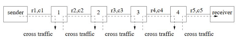
Figure 2.7: A multi-hop network with multiple token bucket shapers
Impact of token bucket shapers Figure 2.12 shows the dispersion rate histograms when we set the token rate r1 of the network in Figure 2.7 to 100 and 250 Mbps, respectively, for the left and right histograms. In both cases, r1 is still the token rate R of the path, and the sending rate of the estimation train λet is set to αC = 350 Mbps. We notice that R is not always the strongest mode, for example in Histogram 2.12(b).
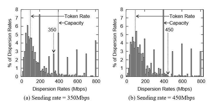
Figure 2.11: The impact of sending rates. Cross traffic = 50%, Burst=1500 bytes, Probing packet=500 bytes
This is demonstrated in Figure 2.11. For example, 350 Mbps is not a mode in His to gram 2.10(b), but it turns to a mode in Histogram 2.11(a), which is obtained using sending rate 350Mbps that is slower than C. As another example, 450 Mbps is not a mode in Histogram 2.10(b), and it is still not a mode in Histogram 2.11(b), which is obtained using sending rate 450 Mbps that is faster than C.
NETWORK PATH CAPACITY COMPARISON WITHOUT ACCURATE PACKET TIME INFORMATION
Design Space and Related Work
The design space shown in Figure 3.1 is based on the required information of probing packets at the receiver. Path Char and Tail Gater estimate the capacity of each individual link in the path using the packet arrival times at the receiver. CapProbe and PBProbe estimate the path capacity using the packet arrival times. BProbe, PBM, and PathRate estimate the path capacity using the packet arrival time differences at the receiver (defined in Section 3.4). Our proposed PathComp relatively compares the path capacities from two senders to the same receiver using the packet arrival sequence number differences at the receiver.
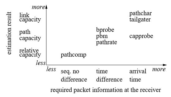
Figure 3.1: The design space of capacity estimation methods
The traditional capacity estimation problem considers the capacity of the narrow link of a single path. For example, for the two paths in Figure 3.2, the traditional capacity estimation problem separately estimates Ca and Cb.
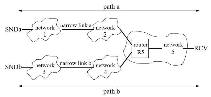
Figure 3.2: Two paths: path a is from sender SNDa to receiver RCV, and path b is from sender SNDb to the same receiver RCV
We study five possible types of cross traffic as illustrated in Figure 3.7, which is very similar to Figure 3.2 and just simplifies each network to a single router. The capacity of each link is chosen to demonstrate the impact of the cross traffic on that link. We emulate this network using our 10Gbps testbed, and each link is emulated by a Linux token bucket filter (tbf).
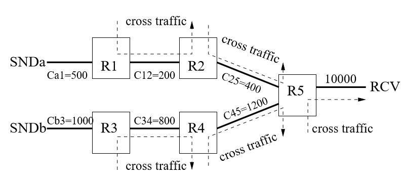
Figure 3.7: Five possible sources of cross traffic. Link capacity unit: Mbps
Preliminary Phase This phase measures the RTT difference △RTT between SNDa RCV and SNDb-RCV as illustrated in Figure 3.19, so that in the next two phases the packets of SNDa and SNDb can overlap with each other. PathComp measures △RTT multiple times, and calculates the mean (denoted by △RTT) and standard deviation (denoted by σ(△RTT)) of measured △RTT values.

Figure 3.19: PathComp has three phrases
RATE LIMITING IN PUBLIC CLOUDS
Azure’s Rate Limiter
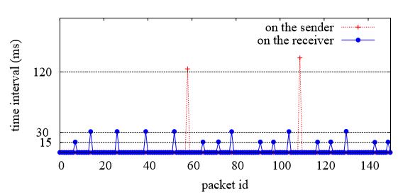
Figure 4.10: Time intervals on sender and receiver side for Azure instance M1
In Azure, M1 uses a Xen-like rate limiter in the network. The reason is the traffic follows a (T, ∆) pattern. Using our UDP probing tool, we measure the time intervals between two consecutive packets on both the sender side and the receiver side as shown in Figure 4.10. The large interval is around 120 ms on the sender side (sleeping period), and on the receiver side it is 15 or 30 ms. Moreover, we find that 6.5 packets are received on average when the interval is 15ms, and 13 packets are received when the interval is 30 ms. Hence, if T = 15 ms, then ∆ = 6.5 packets; if T = 30 ms, then ∆ = 13 packets.
Google’s Rate Limiter
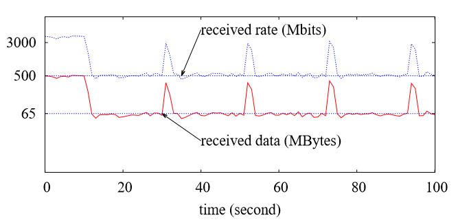
Figure 4.9: Iperf Result for Google instance G1
G1 uses a Linux tbf-like rate limiter in the network. The conclusion is based on the fact that the iperf result demonstrates that the rate follows (P, R, b) pattern. As shown in Figure 4.9 about an iperf result of G1 instance, the peak rate is P = 3.2 Gbps at beginning, and later changes to R = 500Mbps. We observe that the peak rate is varied when the receiver changes from n1-standard-2, to n1-standard-4, and n1-standard-8, The peak rate changes from 1.5 Gbps to 2.2 Gbps, and 3.2 Gbps. This is due to that a high performance instance can send data at a high speed.
CONCLUSION
In this chapter, we described how rates are limited in public clouds. We measure the three most popular public clouds, Amazon EC2, Google Compute Engine, and Microsoft Azure, and found two main rate limiting methods. First, VM scheduling itself can shape the traffic, proven by the observations from the Azure instances. Second, rate limiters are used in the network paths to shape traffic.
We considered two main rate limiters, the Linux tbf-like rate limiter and the Xen-like rate limiter. These rate limiters are found in the public clouds. Our data was measured in September of 2014. This is a little different from our measurement in June 2014, as the cloud providers update their networks and instances.
It is also possible that our result would be different from other studies done in the future. Even so, our measurement can be used to compare the degree to which public clouds improve their networking performance.
Source: University of Nebraska-lincoln
Author: Ertong Zhang