ABSTRACT
Chirp signals can achieve a high range resolution without sacrificing SNR or maximum range, making them a strong candidate for use in radar and sonar applications. Chirp signals are also power efficient and resistant to interference, making them well suited for communication applications as well. The proposed digital high chirp rate receivers will showcase the use of digital instantaneous frequency measurement (IFM) devices for high chirp rate measurement.
The receivers are paired with a high resolution time-of-arrival algorithm, capable of detecting the TOA and TOD of a pulse with an average error of less than 2ns. The high resolution pulse detector is vital for the measurement of high chirp rate, short pulse duration chirp signals when no a priori knowledge of the signals or operating environment is available. Three different receivers were designed and implemented in order to target three different applications: linear chirp signals, nonlinear chirp signals, and linear chirp signals with varying pulse widths.
In addition to the digital IFM and TOA algorithm, a high rate 43-tap Hilbert Transform was implemented via an FIR filter in order to convert incoming real data from the ADC into its complex signal representation. All three designs were synthesized and successfully tested on a Xilinx Virtex 6 SX475 FPGA which is paired with a Calypso 12-bit ADC sampling at 2.56GHz. All three receivers run at a rate of 320MHz and can measure chirp rates up to 1180MHz in 400ns.
The designs boast an overall detection rate of greater than 97% with a false alarm rate of 10-7 and achieve a frequency measurement error of less than 1% for both chirp rates and carrier frequencies. The receivers can successfully detect and measure chirp signals and stationary carrier frequencies with SNRs 5dB and higher. The largest design, the digital nonlinear chirp receiver only utilizes 13% of the Virtex 6 SX475 FPGA board.
DESIGN FLOW AND PROTOTYPING HARDWARE
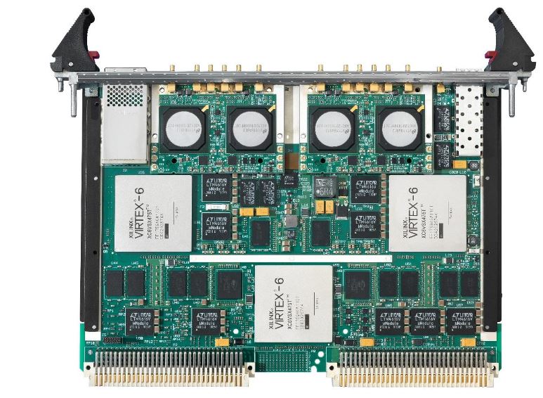
Figure 4–Calpyso Virtex 6 SX475 FPGA pair ed with 3.6 GSPS 12-bit ADC.
The target device for this research is a Virtex 6 SX 475 FPGA paired with a Calypso 12-bit ADC, which was developed by Tekmicro. The ADC is capable of sampling at a rate of up to 3.6GSPS, but was configured to use a sampling rate of 2.56GSPS for all the digital chirp receivers in this dissertation. The Tekmicro device can be seen in Fig. 4.
TIME-OF-ARRIVAL DETECTION OF CHIRP SIGNALS
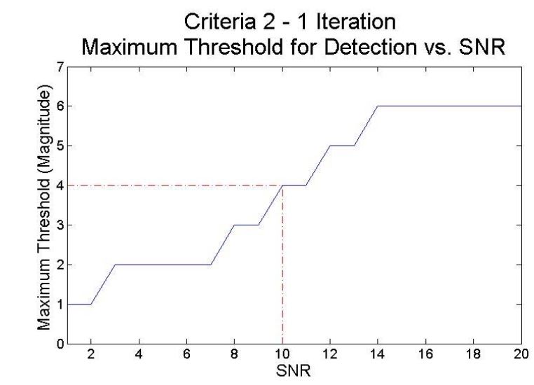
Figure 10–Criteria 2–1 iteration plot of 90% detection rate and false alarm rate thresholds
The same plots were generated to measure the performance of criteria 2, which operates using the maximum magnitude value within an 8-sample block. An additional constraint was added to criteria 2, which sets the minimum number of occurrences required within an 8-sample block. Fig. 10 shows the 90% detection rate threshold vs.SNR for criteria 2 when only 1 magnitude occurrence is required.
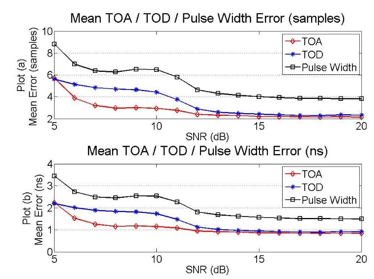
Figure 22–TOA algorithm TOA/ TOD/Pulse Width performance for SNRs from 5dB to 20dB
The TOA model achieves an average TOA error of 2.76 samples (1.07 ns), an average TOD error of 3.45 samples (1.35ns), and an average pulse width error of 5.32 samples (2.08ns) for SNRs from 5dB to 20dB. The temporal resolution provided from the TOA model is well below the 10ns requirement and is acceptable for use with high chirp rate signals with short pulse durations. The plot of TOA/TOD and pulse width measurement error can be seen in Fig. 22.
DIGITAL IMPLEMENTATION OF HILBERT TRANSFORM FOR WIDE BANDWIDTH SIGNALS
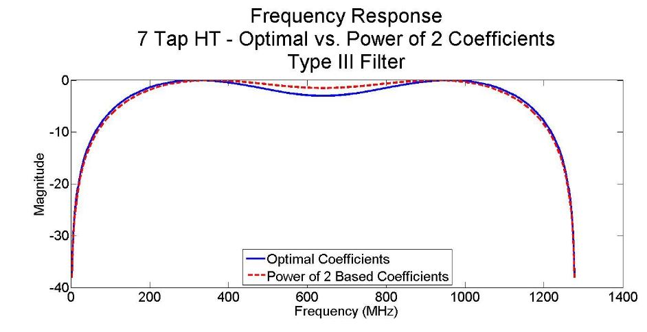
Figure 26-Frequency response of 7-tap type III Hilbert Transform
As the number of filter coefficients are increased, a wider passband region can be obtained at the expense of increased filter implementation complexity. Fig. 26 shows the frequency response comparison for a 7 tap HT when the optimal coefficients are used vs.using powers of 2 based coefficients.
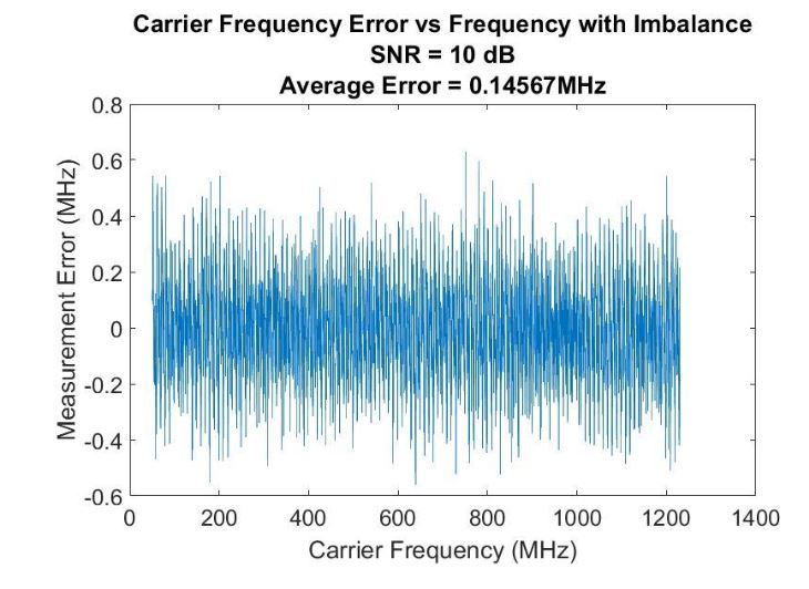
Figure 35–Digital IFM frequency measurement error when the imbalance from the Hilbert Transform is not corrected
The effect of this imbalance on the digital IFM’s measurement performance was simulated in Matlab. Carrier frequencies ranging from 50MHz up to 1230MHz were measured using the digital IFM with the imbalance present and were measured again after applying the correct ion factor previously mentioned. Fig. 35 shows the measurement performance at an SNR of 10dB when the imbalance is present.
DIGITAL INSTANTANEOUS FREQUENCY MEASUREMENT FOR CHIRP MEASUREMENT
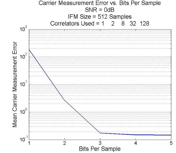
Figure 41-Digital IFM frequency measurement performance vs.number of bits per sample
The phase measurement resolution of the IFM can also be improved by increasing the amount of data stored within each sample. Fig. 41 shows the average frequency measurement error of the IFM as the number of bits per sample is increased.
Again, the entire frequency range from 50MHz up to 1230MHz was tested for each point on the graph. The SNR for all signals was kept constant at 0dB and the correlators. The IFM collected a total of 512 samples for each simulation. It can be seen that the largest improvement is gained from increasing the number of bits from 1 to 2.
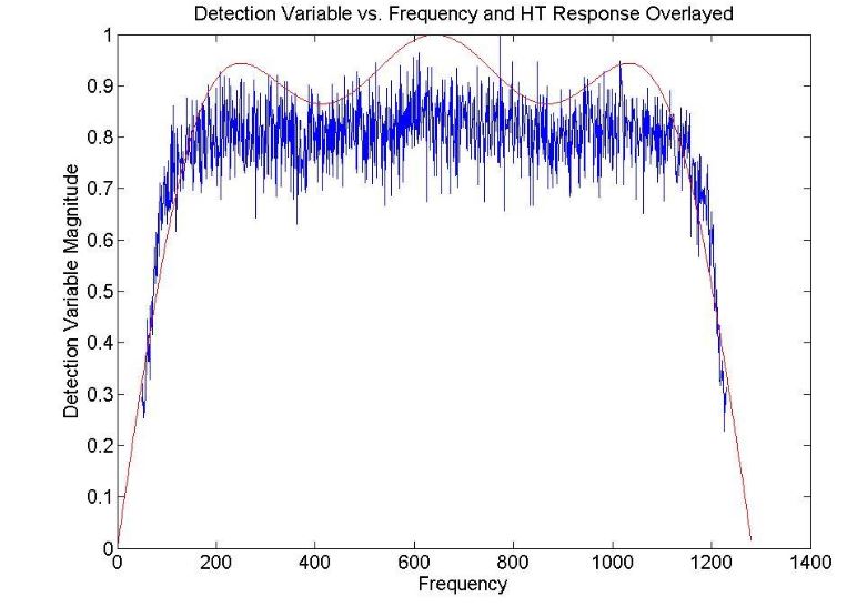
Figure 47-Frequency response of the digital IFM detection variable when an 11-tap Hilbert Transform is utilized
An important aspect to the detection variable is that its frequency response is directly affected by the frequency response of the Hilbert Transform. For this reason, the determination of any detection thresholds should only be determined when the HT and IFM are operating tog ether. The relationship between the HT response and the detection variable can be seen in Fig. 46 and 47 respectively.
LINEAR CHIRP RECEIVER
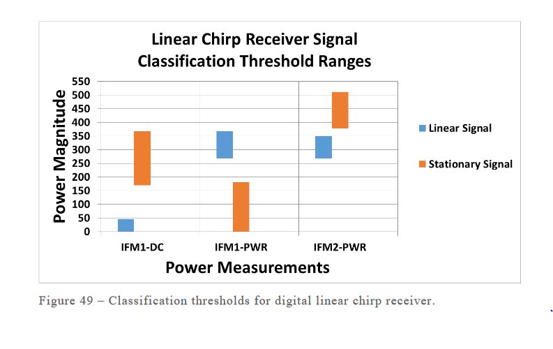
Figure 49–Classification thresholds for digital linear chirp receiver
Fig. 49 shows the entire range of values that each power measurement assumed during the simulations for each of the signal types. Linear chirp signals exhibit DC power measurements from the first IFM which are typically very small in magnitude. As a result, the power measurement from the first IFM is typically significant in magnitude.
NONLINEAR CHIRP RECEIVER
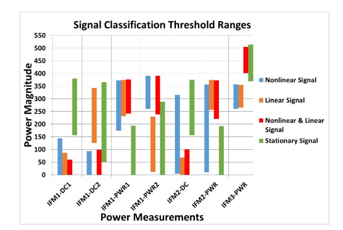
Figure 51–Classification thresholds for the digital nonlinear chirp receiver
Each signal type uses its own set of thresholds for each power and frequency measurement. If all of the measurements fall within an acceptable range for a given signal type, the signal will be classified as that type. If the measurements do not meet all the criteria for any signal type, the receiver reports no output. A lower and upper threshold is stored in the receiver for each measurement and signal type combination. Fig. 51 shows the acceptable range for each measurement and signal type.
VARIABLE CHIRP RECEIVER

Figure 52–Digital variable chirp receiver data flow
The chirp rate and carrier frequency can be measured simultaneously, however, a frequency correction based on the measured pulse width will need to be applied to both measurements. The correction factor for the carrier frequency is dependent on the measurement of the chirp rate. An abstract data flow for the variable chirp receiver can be seen in Fig. 52.
PERFORMANCE EVALUATIONS
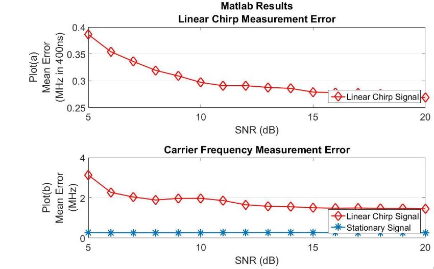
Figure 53–Linear chirp receiver Matlab based frequency measurement performance
Fig. 53 plot (a) shows the mean error in MHz per 400ns for linear chirp rate measurement error. Plot (b) shows the mean carrier frequency error in MHz for both linear chirp signal and stationary signal types. Table XI summarizes the performance of the linear chirp receiver for all signal types.
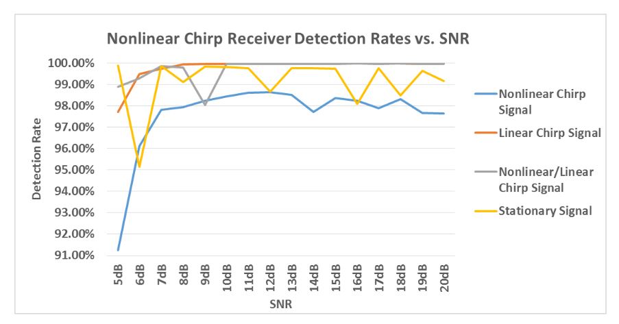
Figure 62-Nonlinear chirp receiver FPGA based detection rates vs. SNR
Fig. 62 shows the detection rates achieved for all four signal types across the tested SNRs. Table XVII shows the average detection rates and also shows that no mis-classification errors were encountered for all 1,380,000 signals tested on the FPGA. The overall detection rates are maintained above 97% for all four signal types.
CONCLUSION
Research Contributions
Measuring high chirp rate, short pulse duration signals is a difficult problem. Ideally, a long pulse duration is desirable to achieve a high SNR and allow for an accurate and reliable frequency measurement. This allows for a large size FFT to be utilized. However, when the pulse duration is very short, the FFT is unable to measure frequencies with a high resolution unless a very high sampling rate is utilized. The difficulty of this problem is further compounded when no a priori knowledge of the signal is available. Typical approaches utilize a matched filter approach, which is a maximum likelihood solution. The research conducted for this dissertation successfully shows a proof of concept, which is able to detect and measure high chirp rate linear and nonlinear signals with no a priori knowledge.
Future Research
The biggest limitation of the three digital chirp receivers is their inability to measure more than one simultaneous signal. This is due to the inherent functionality of the digital IFM, which takes a single discrete phase measurement. It should be possible to measure more than one simultaneous signal by utilizing multiple channelized receivers, for example one receiver operates from 50MHz up to 1,230MHz and a second receiver operates from 1,33 0MHz up to 2,51 0MHz.
Source: Wright State University
Author: Benson Ray Stephen